


COCOMO Model in Software Engineering: Comprehensive Guide
Updated on : 05 May 2025

Image Source: google.com
Table Of Contents

- 1. Introduction
- 2. Historical Context and Evolution
- 3. Project Classification System
- 4. Three-Level Estimation Hierarchy
- 5. Mathematical Foundations
- 6. Cost Driver Adjustments
- 7. Phase-Wise Effort Distribution
- 8. Step-by-Step Calculation Process
- 9. Real-World Implementation Example
- 10. Strengths vs Limitations
- 11. Comparison with Alternative Models
- 12. Modern Tools and Extensions
- 13. Implementation Best Practices
- 14. FAQs
- 15. Conclusion
Table Of Contents

Introduction
COCOMO (Constructive Cost Model)Model in Software Engineering: a software cost estimation model developed by Barry W. Boehm in 1981. It helps estimate the effort, cost, and time required to develop a software project based on the size of the software, usually measured in Kilo Lines of Code (KLOC).
Key Objectives:
-
Estimate the effort (person-months).
-
Predict the project duration.
-
Assist in project planning and budgeting.

Image Source: google.com
| ✅ Advantages | ❌ Disadvantages |
|---|---|
| Provides quick, rough estimation for planning | Less accurate due to ignoring key cost drivers |
| Easy to implement and understand | Does not account for project complexity or environment |
| Intermediate model increases accuracy with cost drivers | Still does not offer phase-wise breakdown |
| Detailed model gives precise phase-wise effort estimates | Complex to implement and maintain |
| Helps in budget and resource planning | Requires extensive data collection for detailed model |
| Supports various project types (organic, semi-detached, embedded) | Each model needs calibration for different environments |
Project Categories in COCOMO:
-
Organic – Small, simple software projects with experienced teams.
-
Semi-Detached – Medium projects with mixed experience.
-
Embedded – Complex projects with tight constraints.
Why COCOMO is Important in Software Engineering:
-
Offers a structured approach to estimation.
-
Helps in resource allocation.
-
Useful for feasibility studies and planning.

Custom mobile apps by Hexadecimal Software, estimated using the COCOMO model.

Historical Context and Evolution
The development of the COCOMO model over time shows how it has evolved to keep up with advancements in software engineering practices:
| Version | Year | Key Improvements |
|---|---|---|
| COCOMO 81 | 1981 | Original waterfall model-based estimation |
| COCOMO II | 2000 | Added object-oriented and spiral model support |
| COCOMO III | 2020 | Integrated DevOps and CI/CD pipelines |
COCOMO 81 (1981):
- This was the original version of the model.
- It was designed for projects using the traditional waterfall model and focused on estimating cost and effort based primarily on the size of the software measured in KLOC (thousands of lines of code).
COCOMO II (2000):
- As software development methods evolved, this updated version introduced support for object-oriented programming, reuse, and spiral development models.
- It also improved estimation accuracy for modern and iterative development approaches.
COCOMO III (2020):
- Reflecting the current software development environment, this version integrated support for DevOps practices, continuous integration/continuous deployment (CI/CD) pipelines.
- Agile methodologies, making it more suitable for today's fast-paced development cycles.
Project Classification System
| Type | Team Size | Innovation Level |
|---|---|---|
| Organic | <5 | Low (routine projects) |
| Semi-Detached | 5-15 | Medium (mixed experience) |
| Embedded | >15 | High (strict requirements) |
Organic Projects:
- These are small and straightforward projects typically handled by teams of fewer than 5 members.
- The work is generally routine, with low levels of innovation.
- An example would be a simple payroll system update.
Semi-Detached Projects:
- These projects are of intermediate complexity, with team sizes ranging from 5 to 15.
- The team usually has a mix of experienced and less-experienced members.
- An example is developing an e-commerce platform.
Embedded Projects:
- These are large, complex systems that operate within strict hardware or software constraints.
- They usually require high innovation and are built by teams of more than 15 people.
- A typical example is avionics software for aircraft.
Three-Level Estimation Hierarchy
| Level | When Used | Inputs Required | Accuracy |
|---|---|---|---|
| Basic | Initial feasibility study | Size in KSLOC | ±30% |
| Intermediate | Requirements finalized | Size + Cost drivers | ±20% |
| Detailed | Detailed design phase | Phase breakdowns | ±5% |
Basic Level:
- This is used during the initial feasibility study, when only a rough idea of the project size is available.
- It requires just the estimated size in Kilo Source Lines of Code (KSLOC) and typically provides an accuracy of around ±30%.
Intermediate Level:
- Used when the project requirements are finalized, this level incorporates both size estimates and various cost drivers (such as required reliability, team capability, and development tools).
- It improves accuracy to about ±20%.
Detailed Level:
- Applied during the detailed design phase, this level breaks down the project into specific phases and includes all cost drivers along with phase-specific effort multipliers.
- It offers the highest accuracy, typically around ±5%.
Mathematical Foundations
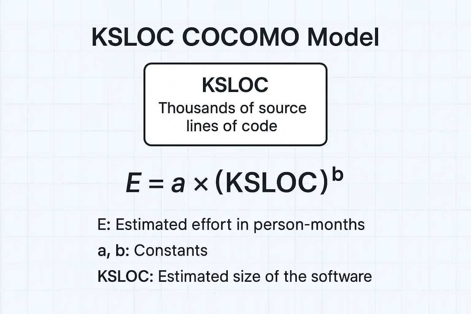
Image Source: google.com
🔹 Effort (E)
This represents the total effort required in person-months:
E = a × (KSLOC)b
- KSLOC: Estimated size of the software in thousands of lines of code.
- a, b: Constants that vary based on the project type (Organic, Semi-Detached, Embedded).
🔹 Duration (D)
This gives the estimated time in months to complete the project:
D = c × (E)d
- E: Effort from the previous formula.
- c, d: Empirically derived constants based on historical data and project category.
🔹 Staff (S)
This is the average number of people needed:
S = E / D
Cost Driver Adjustments

Image Source: google.com
In Intermediate COCOMO, estimates are refined using 15 cost drivers, which adjust the effort based on various project-related attributes. These drivers are grouped into four main categories, each with specific factors and associated multipliers that influence the final effort:
| Driver Category | Example Factors | Multiplier Range |
|---|---|---|
| Product | Reliability, Complexity | -0.6499999999999999 |
| Platform | Memory constraints, Volatility | -0.43000000000000005 |
| Personnel | Experience, Continuity | -0.4900000000000001 |
| Project | Process maturity, Tools | -0.35 |
Product Factors
These are characteristics related to the software product itself — what you're building.
Examples:
-
Required reliability: For example, software used in medical or aerospace systems must be highly reliable.
-
Product complexity: A simple CRUD app is less complex than an AI-based image recognition system.
Multiplier Range: 0.75 to 1.40
-
If the product has low complexity or low reliability needs, the multiplier is low → less estimated effort.
-
If it's highly complex or must be extremely reliable, the multiplier is high → more effort required.
Platform Factors
These relate to the hardware and software environment where the product will run.
Examples:
-
Memory constraints: If the software needs to run on a low-memory device, developers must optimize code more.
-
Platform volatility: Frequent changes in the OS, hardware, or tools can lead to rework.
Multiplier Range: 0.87 to 1.30
-
Stable, resource-rich platforms reduce effort (lower multiplier).
-
Tight constraints or unstable platforms increase effort (higher multiplier).
Personnel Factors
These focus on the skills, experience, and organization of the development team.
Examples:
-
Experience levels: Developers familiar with the language, tools, or domain will be more productive.
-
Team continuity: Stable teams (low turnover) work more efficiently together.
Multiplier Range: 0.85 to 1.34
-
Skilled and stable teams require less effort.
-
Inexperienced or frequently changing teams need more effort to complete the same tasks.
Project Factors
These involve management practices, tools, and methodologies used during development.
Examples:
-
Maturity of the process: Teams following a structured, well-defined development process (like CMMI Level 5) are more efficient.
-
Use of tools and methods: Using effective project management tools, automated testing, or modern DevOps practices helps reduce manual effort.
Multiplier Range: 0.91 to 1.26
-
Better tools and processes → lower effort.
-
Poor or no formal processes → increased effort due to miscommunication, errors, or delays.
You Might Also Like

React vs Angular: Which Framework Should You Choose in 2025?
By Hexadecimal Software Team
on 2025-04-09

Steps in SDLC Life Cycle: Plan, Analyze, Design, Build, Test
By Hexadecimal Software Team
on 2025-04-16

REST API vs SOAP: Protocol Comparison for Web Services
By Hexadecimal Software Team
on 2025-04-12

Full Stack Guide: MERN, MEAN and More Explained for Devs
By Hexadecimal Software Team
on 2025-05-01
Phase-Wise Effort Distribution
| Phase | Effort % | Key Activities |
|---|---|---|
| Requirements | 6% | Stakeholder interviews, SRS creation |
| Design | 19% | Architecture diagrams, DB design |
| Implementation | 62% | Coding, unit testing |
| Validation | 13% | System integration, UAT |
Requirements Phase (6%)
-
Effort Allocation: 6% of the total effort
-
Activities: Involves stakeholder interviews, defining functional and non-functional requirements, and preparing the Software Requirements Specification (SRS).
Design Phase (19%)
-
Effort Allocation: 19%
-
Activities: Includes system and software architecture design, database design, and creation of high- and low-level design documents.
Implementation Phase (62%)
-
Effort Allocation: 62%
-
Activities: Focuses on coding, unit testing, and integrating modules—this is the most resource-intensive phase.
Validation Phase (13%)
-
Effort Allocation: 13%
-
Activities: Involves system integration testing, User Acceptance Testing (UAT), and final quality assurance before deployment.
For Flutter App Development Services with Hexadecimal Software
Build beautiful cross-platform apps—fast—with Hexadecimal Software and Flutter.
Step-by-Step Calculation Process
1. Estimate Size
-
Determine the project size in KSLOC (Kilo Source Lines of Code).
-
This can be based on past projects, function points, or early requirement specs.
2. Select the Model Type
Choose the appropriate COCOMO model based on the project characteristics:
-
Organic – Simple, familiar projects with small teams
-
Semi-Detached – Medium complexity and mixed experience teams
-
Embedded – Complex, tightly constrained systems
3. Compute Base Effort
Use the basic formula:
E = a × (KSLOC)b
- E = Effort (in person-months)
- KSLOC = Thousands of source lines of code
- a, b = Constants based on project type (Organic, Semi-Detached, Embedded)
4. Adjust Effort
Multiply the base effort by the Effort Adjustment Factor (EAF):
Adjusted Effort = E × EAF
- E = Base effort (from the previous step)
- EAF = Product of all relevant cost driver multipliers
5. Calculate Duration
Use the formula:
D = c × (E)d
- D = Duration in months
- E = Adjusted effort
- c, d = Constants based on the project type
6. Determine Staffing
Calculate the average number of people needed:
S = E / D
- S = Average staffing
- E = Adjusted effort
- D = Duration in months
Real-World Implementation Example
Project: Hospital Management System (35 KSLOC, Semi-Detached)
- Base Effort = 3.0 * (35)^1.12 = 3.0 * 47.85 = 143.55 PM
- Adjusted Effort = 143.55 * 1.15 (average cost drivers) = 165.08 PM
- Duration = 2.5 * (165.08)^0.35 = 2.5 * 5.01 = 12.53 months
- Staffing = 165.08 / 12.53 ≈ 13 developers
Strengths vs Limitations
Accuracy
-
Advantage: It is based on historical project data, making its estimates data-driven and reliable when applied correctly.
-
Challenge: The accuracy heavily relies on having precise estimates of lines of code (LOC) early in the project, which can be difficult during the initial stages.
Flexibility
-
Advantage: COCOMO allows customization through cost drivers, enabling it to adapt to different project types and environments.
-
Challenge: It assumes that requirements are stable, which might not hold true for agile or evolving projects.
Usability
-
Advantage: The model provides a clear and structured mathematical framework, making it easy to understand and implement.
-
Challenge: For best results, COCOMO needs to be calibrated to specific organizations using their past project data, which may not always be readily available.

Need a powerful web app? Hexadecimal Software builds it to perform.
Comparison with Alternative Models
| Model | Strength | Weakness |
|---|---|---|
| Function Points | Language-independent, useful across platforms. | Subjective complexity, dependent on estimator's experience. |
| Agile Estimation | Adapts to changing requirements. | Lacks precision and mathematical rigor. |
| Machine Learning | Effective at pattern recognition in data. | Requires large datasets for training. |
For AI/ML Services with Hexadecimal Software
Unlock the power of AI and machine learning with Hexadecimal Software to drive smarter solutions and innovations.
Modern Tools and Extensions

Image Source: google.com
| Tool | Platform | Key Feature |
|---|---|---|
| COCOMO II | Windows/Linux | Reuse model extension |
| SEER-SEM | SaaS | AI-driven adjustments |
| SLIM Estimate | Cloud | Monte Carlo simulation |
COCOMO II
-
Platform: Available for Windows/Linux
-
Key Feature: Offers a reuse model extension, which helps adjust estimates based on reused software components and their complexity.
SEER-SEM
-
Platform: SaaS (Software as a Service)
-
Key Feature: Uses AI-driven adjustments to refine estimates based on historical data and evolving project characteristics.
SLIM Estimate
-
Platform: Available on the Cloud
-
Key Feature: Uses Monte Carlo simulation to provide probabilistic estimates, allowing users to assess a range of possible project outcomes.
Implementation Best Practices
- Calibrate Constants: Adjust a,b,c,d using historical project data
- Combine Techniques: Use with Function Points for requirements-phase estimates
- Update Regularly: Recalibrate every 18 months for technology changes
- Document Assumptions: Clearly state size estimation methodology
Connect with Hexadecimal Software for COCOMO-accurate cost estimation.
Need precise software cost estimates? Hexadecimal Software delivers with COCOMO-driven accuracy.
FAQs
Q1: How does COCOMO handle distributed teams?
A: Adjust the "Multi-site Development" cost driver (0.93-1.22 multiplier).
Q2: What's the alternative to lines of code?
A: Use Function Points converted to LOC via language conversion factors.
Q3: How accurate is COCOMO for agile projects?
A: COCOMO III includes a 0.91-1.11 "Agile Process" multiplier.
Q4: Can COCOMO estimate maintenance efforts?
A: Yes, annual maintenance = 15-20% of development effort.
Q5: How to estimate KSLOC early in projects?
A: Use analogy-based estimation or Delphi wideband technique.
Q6: What's the learning curve for COCOMO?
A: 2-3 weeks for basic proficiency, 3 months for expert calibration.
Conclusion
In conclusion, the COCOMO model is a reliable tool for estimating software effort, duration, and staffing, tailored to different project types. It’s data-driven but requires accurate input. Other models like Function Points and Agile Estimation offer flexibility, while tools like SEER-SEM and SLIM Estimate use AI and simulations for dynamic estimates. The best choice depends on the project’s needs and team experience.


Buy, Sell & Rent Properties – Download HexaHome App Now!

Find your perfect home, PG, or rental in just a few clicks.

Post your property at ₹0 cost and get genuine buyers & tenants fast.

Smart alerts & search helps you find homes that fit your budget.
Available on iOS & Android
Available on iOS & Android


Scan to Download our App
Available on iOS & Android – Download Now!

A Product By Hexadecimal Software Pvt. Ltd.